Introduction
In this post, let’s try to understand the geometric intuition behind the Local To World Matrix and try to make sense of matrix multiplication a bit better through a simple illustration.
– Why exactly are we multiplying row ‘i’ of matrix A with column ‘j’ of matrix B to get an element ‘Rij‘?
This post is going to talk a lot. So, please bear with it. 🙂
Matrix Multiplication: Geometric Intuition
For a refresher on matrix multiplication, I recommend going though this article. In summary, multiplication of matrix can be interpreted as Dot product of row ‘i’ of matrix A with column ‘j’ of matrix B to get the element ‘Rij‘.
If you ever wondered why exactly multiplications are done this way and what’s the geometric interpretation behind it, this article is for you! 🙂
Here are the assumptions I’ve defined:
– All the matrices and vectors in this article are represented using Column-Major notation.
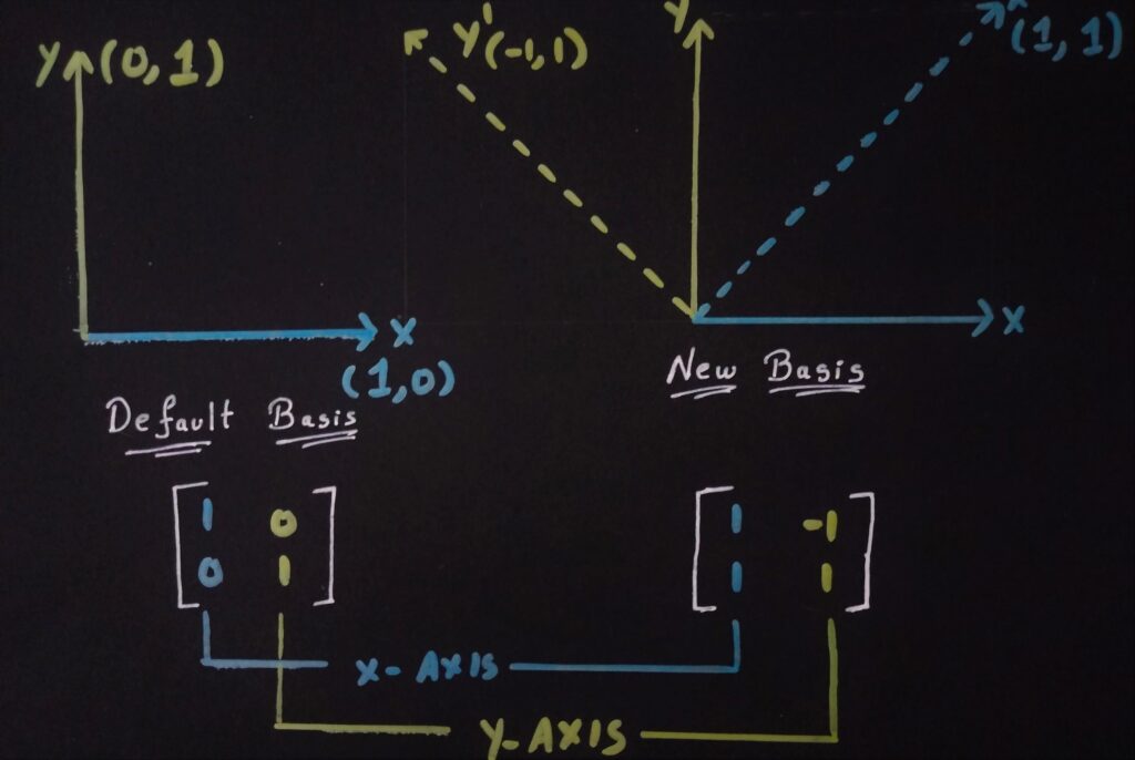
– Our basis vectors for “World-Space” coordinate system are each represented by a column in a square matrix. Let this matrix be represented by ‘W‘ (Default Basis).
– Let’s assume a new set of 2D basis vectors(not necessarily orthonormal). If a point is represented relative to this new basis, we are representing the point in local space (New Basis).
– A 2D point P(2, 3) as an example.
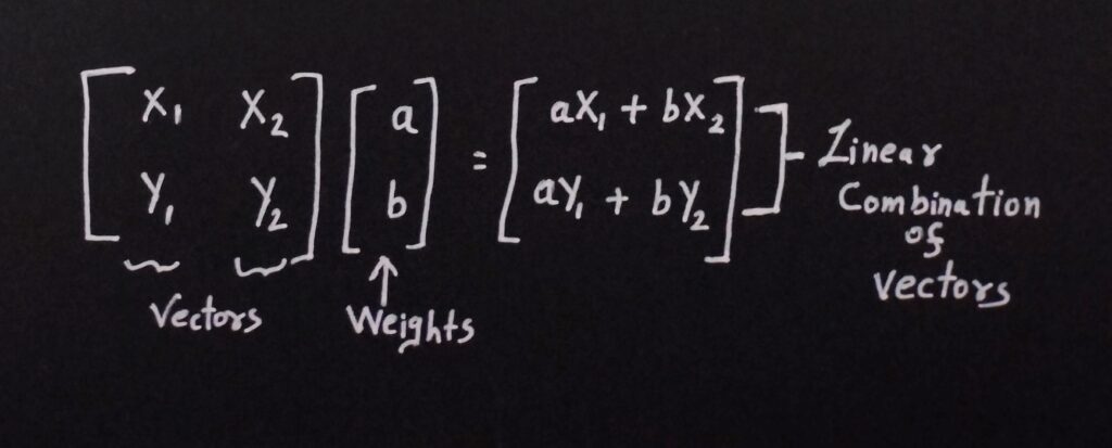
If we look at a generic multiplication, we can see that the result is a “linear combination” of rows of matrix A with the weights coming from matrix B.
Now, if we replace the matrix A with our Default Basis and perform the multiplication, we end up at 2 units to right and 3 units up. Understanding what’s happening here is vital to making sense of geometric interpretation of matrix multiplication.
On expanding multiplication, we get following equations:
– (1)(2) + (0)(3) = 2 = P’.X
– (0)(2) + (1)(3) = 3 = P’.Y
Everything is beautiful in our Default Basis. Our Y-axis vector doesn’t have an X component to add weight to P’.X!
Similarly, X-Axis doesn’t have Y-Component to add any weight to P’.Y!
As a result, we cleanly end up at the location we expect to.
Now, what if the basis vectors are not so clean(like our ‘New Basis’)?
Another intuitive point to note is that this “New Basis” is represented in terms of our Default Basis.
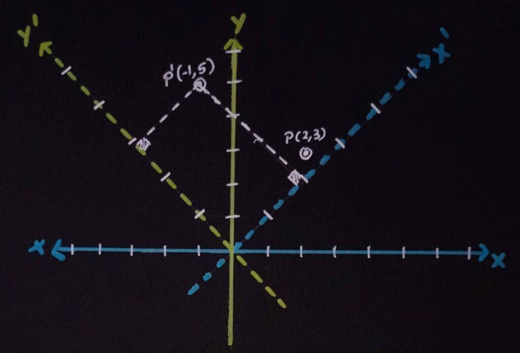
If we apply the same matrix multiplication to this new basis and the same point, we get this:
(1)(2) + (-1)(3) = -1 = P’.X
(1)(2) + (1)(3) = 5 = P’.Y
What exactly is happening here? What does this multiplication imply?
When doing the same calculation with Default Basis, we started and ended with a same point.
Now, with our New Basis, the point (2, 3) represents the location in New Basis’ coordinate system. When the matrix transformation is applied, we are transforming the point from New Basis’ space to Default Basis’ coordinate space.
Local To World Space Intuition:
– To get to point (2, 3) in any coordinate space, we move 2 units right and 3 units up.
– We have represented New Basis in terms of Old basis.
In terms of default basis, 2 units right in New basis is represented by: (1, 1) * 2 = (2, 2).
In terms of default basis, 2 units up is represented by: (-1, 1) * 3 = (-3, 3).
Sum of both these vectors gives our World-Space location: (-1, 5) !!! We simplified the issue from confusing matrices to simple vector addition 😛
In the end, matrices are just glorified representation of linear combination of Basis Vectors !!
There’s one last thing to think about. Why is the matrix multiplication a dot product of rows and columns?
If we look at mapping points in our default basis, P.X and P.Y can be viewed as projections on X(1,0) and Y(0,1) axes respectively.
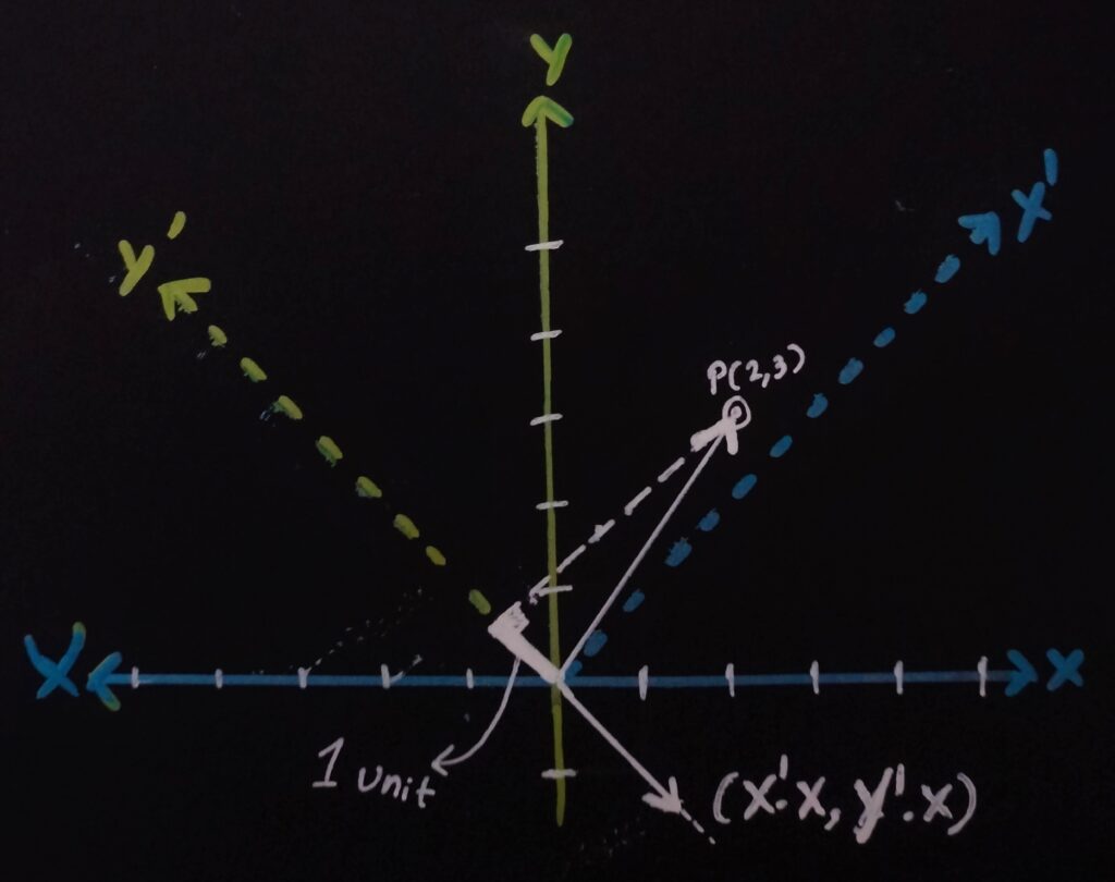
Now, what vector should we project on to get the World-Space coordinates of a local position in New Basis?
– Looking at matrix multiplication, we have P’.X = (X’.X*P.X) + (Y’.X * P.Y). X components of both X’ and Y’ contributes to the final result P’.X in world space.
– A new vector with (X’.X, Y’.X) will be the one that we should project on to get P’.X.
– This can be thought of as vector obtained through the addition of (X’.X, 0) and (0, Y’.X).
– The final vector obtained implies that: X component of X’ is added only along world’s X axis. X component of Y’ is only added along world’s Y axis.
– It’s the same for P’.Y.
A matrix transformation is very simple to learn, but the intuition behind it is quite magical. I apologize if what you read seemed redundant.
Hope this makes you a bit wiser than yesterday! 🙂